Learning how to manipulate and visualise protein structures

Demo Step 7: Detailed interface analysis
Many chemical interactions stabilise polypeptides. Let’s have a look at the interface of our models – let’s start with the relaxed version of our model of rank 1: Is the interface plausible? Does it have strong contacts? Is it stable? Have a look at:
A quick reminder below of the forces that go on in proteins and protein complexes:
| Interaction | Distance dependence | Typical distance | Free energy (some orders of magnitude) |
|---|---|---|---|
| Covalent bond | – | 1.5A | 356kJ/mole |
| Hydrogen bond | Donor (e.g. N) and acceptor (e.g. O) atoms <3.5 A | 3A | 2-6kJ/mole in water |
| Disulfide bond | – | 2.2A | 167kJ/mole |
| Salt bridge | Donor (e.g. N) and acceptor (e.g. O) atoms <3.5 A | 2.8A | 12.5-17kJ/mole |
| Long-range electrostatic interaction | Depends on dielectric constant of medium. Screened by water. 1/r dependence | Variable | Depends on distance & environment. |
| Van der Waals interaction | Short range. Falls off rapidly beyond 4A separation. 1/r^6 dependence | 3.5A | 4kJ/mole depending on the size of the group |
Hydrogen bonds and salt bridges
To detect H-bonds and Salt bridges in your model or at the interface:
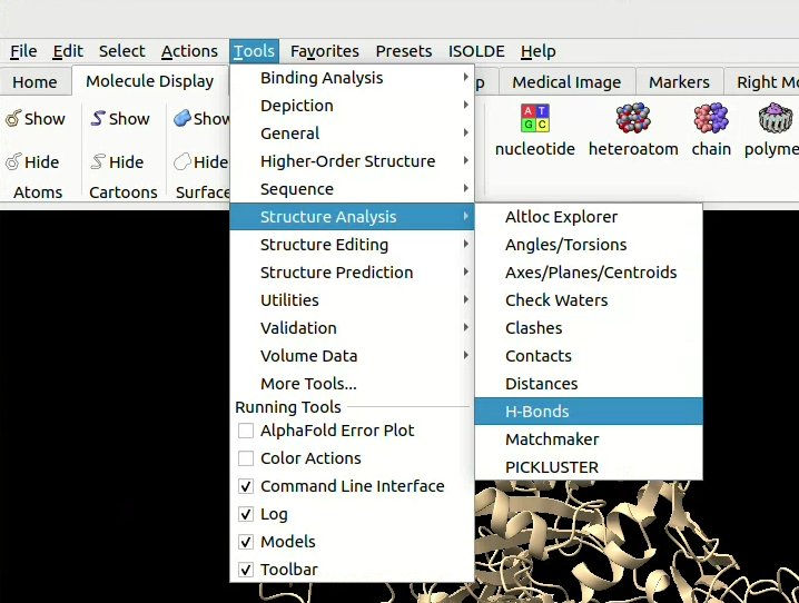
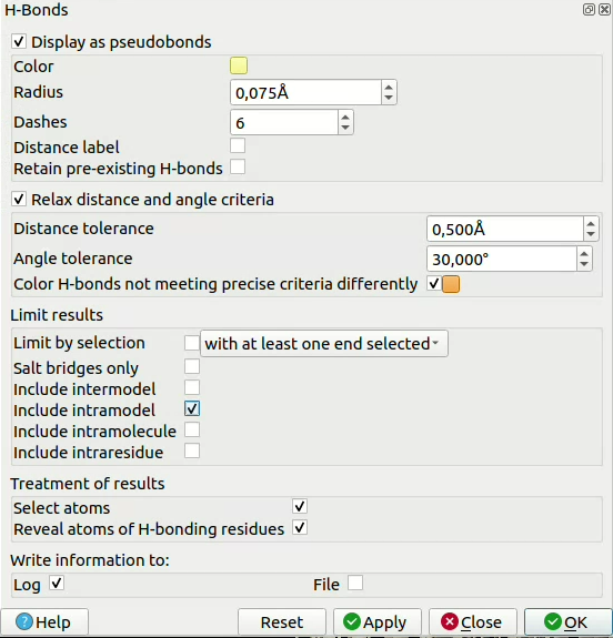
![]() click on Tools > Structure Analysis > H-bonds, then select the parameters you want. You can, for example, relax the constraints on angles and distances to allow for imperfect models. You can also define here if you want to restrict yourself to bonds between two different chains (“Include intramodel” ticked and the rest unticked) or if you would like to include intermolecule bonds too.
click on Tools > Structure Analysis > H-bonds, then select the parameters you want. You can, for example, relax the constraints on angles and distances to allow for imperfect models. You can also define here if you want to restrict yourself to bonds between two different chains (“Include intramodel” ticked and the rest unticked) or if you would like to include intermolecule bonds too.
If you ticked “Select atoms” above, you can easily add the labels of the residues involved in H-bonds and Salt bridges if you go in Tools > Actions > labels, then select the label type you want (e.g. Chain, code, number ).
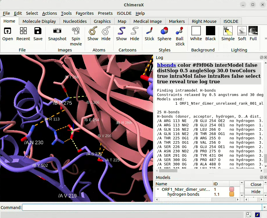
![]() in-line you can use the hbonds command to calculate H-bonds and/or Salt bridges, for example:
in-line you can use the hbonds command to calculate H-bonds and/or Salt bridges, for example:
To detect all H-bonds with ±0.5 Å distance tolerance and ±30° angle tolerance between chains of model #1:
hbonds #1 intraModel true interModel false intraMol false intraRes false distSlop 0.5 angleSlop 30.0 color yellow twoColors true select true reveal true log true name hbonds_model1
To then colour the previous selection by chain and heteroatom:
color sel bychain
color sel byhetero
To add labels to the previous selection:
label sel text “/{0.chain_id} {0.label_one_letter_code} {0.number}{0.insertion_code}”
![]() Click here for more information on the hbonds command line options.
Click here for more information on the hbonds command line options.
To go a bit further…
There are ways of creating home-made functions in ChimeraX (like ChimeraX’s hbonds, color or label commands that you’ve seen previously). They are called aliases. Below is an example which will create the check_interface command, which will put structures in cartoon style, colour them by chain, show the interface residues as sticks and finally calculate the hbonds and the salt bridges and show them in 2 different colours (yellow and lime):
alias check_interface show $1 cartoons; delete H; color $1 bychain; select $1/$2 :<4.5 & $1/$3 | $1/$3 :<4.5 & $1/$2 residues true; show sel atoms; color sel byhetero; hbonds $1/$2 restrict $1/$3 distSlop 0.5 angleSlop 30.0 color yellow twoColors true reveal true log true; hbonds $1/$2 restrict $1/$3 distSlop 0.5 angleSlop 30.0 color lime reveal true log true saltOnly true name salt_bridges; view sel clip true; ~select;
Electrostatics & hydrophobicity
![]() click on the Molecule Display tab in the Menu bar, then select “electrostatic” or “hydrophobic” in the Coloring section to colour your model by electrostatic charges or hydrophobicity.
click on the Molecule Display tab in the Menu bar, then select “electrostatic” or “hydrophobic” in the Coloring section to colour your model by electrostatic charges or hydrophobicity.

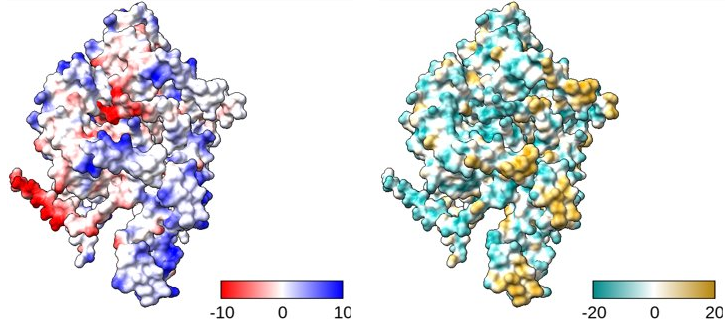
![]() in-line you can use the coulombic and mlp commands to colour by electrostatics and hydrophobicity respectively, for example:
in-line you can use the coulombic and mlp commands to colour by electrostatics and hydrophobicity respectively, for example:
coulombic #1 & protein key true
To plot the electrostatics of all protein elements in model #1. As key is true, it’ll also open up a dialog box to define the colour gradient.
mlp #1 & protein key true
To plot the hydrophobicity of all protein elements in model #1. As key is true, it’ll also open up a dialog box to define the colour gradient.
Sequence conservation
![]() click on the Home tab in the Menu bar, then select “Open” and upload the multiple sequence alignment (MSA) file outputted by AlphaFold in fasta format. This will open an additionnal pane with your MSA. Right click on it, go in Structure > Associations… to select the models and chains the MSA covers.
click on the Home tab in the Menu bar, then select “Open” and upload the multiple sequence alignment (MSA) file outputted by AlphaFold in fasta format. This will open an additionnal pane with your MSA. Right click on it, go in Structure > Associations… to select the models and chains the MSA covers.
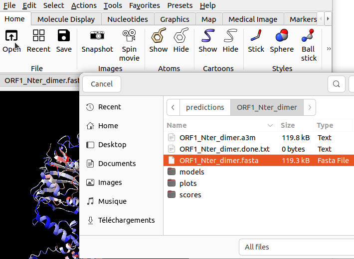
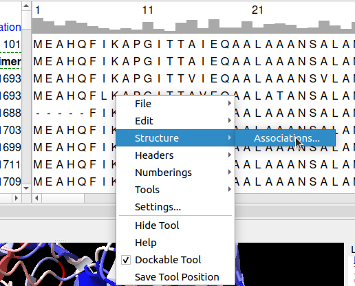
Then to colour your model according to the conservation, you’ll have to pass by the command line like so to colour model #1:
color byattr r:seq_conservation #1
An example of a more complete command to color in the (-2,3) range and add a color bar (cf. key true):
color byattr r:seq_conservation #1 palette cyanmaroon range -2,3 novalue silver key true
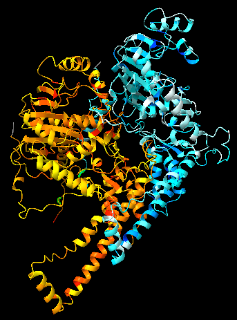
An example to colour chains A & B with two different colours scales:
color byattr r:seq_conservation #1/A palette yellow:red range -2,3 novalue silver key true;
color byattr r:seq_conservation #1/B palette white:cyan:blue range -2,3 novalue silver key true
The above course material is under CC-BY-SA license.